Next: Exercise Up: Linear Differential Equations Previous: Linear Differential Equations Contents Index
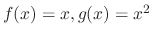
The differential equation of the form
 is called the coefficient function.
 is called the input function.
If
 , then the differntial equation is called the homogeneous equation.
We denote the left-hand side as  . Then the differential equation is expressed as

 is called the differential operator and has linearlity. That is for any solutions
 and constants
 ,
,
We review the vector space.
A sum of two vectors A and B is expressed as A  B and is equal to the diagonal of the parallelogram formed by A and B.
1. A sum of two vetors is a vector (closure)
2. For any vectors A and B,A+B = B+A (commutative law)
3. For any vectors A,B,C, (A+B)+C = A+(B+C) (associative law)
4. Given any vector A, there exists a vector 0 satisying A+0 = A (existence of zero)
5. Given any vector A, there exists a vector B satisfying A+B = 0 (existence of inverse)
6. A scalar multiplication of a vector is a vector
7. For any real numbers  and
and  , (A) = (
 )A (associative law)
8. For any real numbers and , (
 )A = A + A and for any vectors A and B, (A+B) = A + B (distributive law)
9. 1A = A; 0A = 0; 0 = 0 (1 is multiplicative identity)
Let  be the set of continuous functions on the interval
  . Let
. Let  be the set of piecewise continuous functions on , 2.1
 is continuous on },
 is piecewise continuous on }.
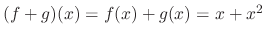
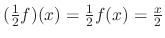
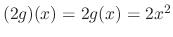
For and  in or , we define the addition on the scalar multiplication as follows:
1.  is a function of
  whose value is equal to
  .
.
2.  is a function of whose value is equal to
 .
.
 , find
 .
.
SOLUTION

with the operation defined above is a vector space. Then the function belongs to is called a vector.
Proof
The solutions of a homogeneous differential equation are differentiable. Thus, the set of solutions are the subset of continuous functions. Then to show is a vector space, it is enough to show the linear combination of the solutions  and
and  is a solution.
Let
is a solution.
Let
 . Then
 |
 |
 |
|
|
 |
||
|
 |
||
|
0 |
 is again a solution.
The set of solutions of homogeneous equation becomes a vector space. So, we call this solution space.
 independent solutions of homogeneous differential equation.
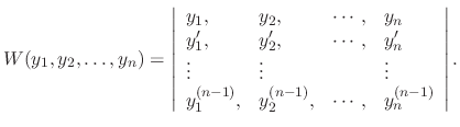
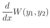
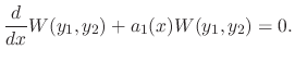
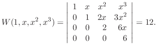
The determinant of the following matrix is called Wronskian determinant. Let  be the solutions of the differential equation. Then
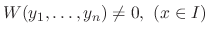
 are the solutions of the homogeneous equation on the interval
 ![$[a,b]$](img46.png) , then
, then
 is either 0 or never 0 0n the interval .
Proof
For  Since
Since  and
and  are solutions of
 , we have
 |
|
 |
|
|
 |
||
|
 |
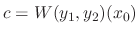
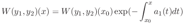
 . Multiplying
  to get
 constant
 . Then
 and
and
are solutions of the homogeneous differential equation on , then the following conditions are equivalent.
 are linearly independent on the interval .
Proof
For , let the linear combination of and be 0. Then
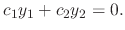 . Then
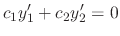
 and
and  .
.
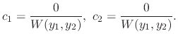
 are linearly independent, then
 . Thus,
 . Conversely, if
, then
. Thus,
are linearly independent
. Conversely, if
, then
. Thus,
are linearly independent
 .
.
SOLUTION
The dimension of the solution space is 3.
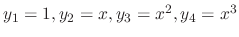 are solutions of the differential equation. So, we need to show they are linearly independent.
 is a solution of
 . Then find the fundamental solution.
SOLUTION
Since
 |
|
 |
|
|
 |
||
|
 |
 implies that
 .
.
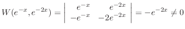
 are fundamental solutions.
 is an particular solution of the-order linear differential equation
 and
and  is the general solution of
  . Then
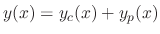 is the general solution of
.
is the general solution of
.
Proof
By the assumption,
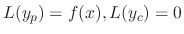 . Now by the linearlity of , we have
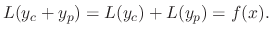
 is a solution of
. Since
is a solution of
. Since  contains constants,
 is the general solution.
is called the complementary solution. By this theorem, if an particular solution of
is found, then to find the general solution, it is enough to find a complementary solution of .
 is an particular solution of
 . Then find the general solution.
SOLUTION
Since
 ,
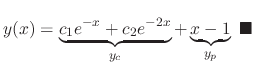
. Also, the complementary solution of is given in example2.2. Thus
,
. Also, the complementary solution of is given in example2.2. Thus
If is given as a sum of  and
and  , then it is better to consider
 and
and
 .
.
 is a solution of
, and
is a solution of
, and  is a solution of
. Then
is a solution of
. Then
 is a solution of
 .
.Proof.

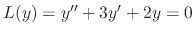
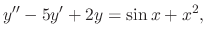
For example, to find the general solution of the differential equation
 of
of
 of
of
 of
of
![\begin{figure}\begin{center}
\includegraphics[width=14cm]{DFQ/Fig0-1.eps}
\end{center}\vspace{-1.6cm}
\end{figure}](img500.png)