Next: System of linear equations Up: Matrix and Determinant Previous: Matrices Contents Index
Solving a system of linear equations is one of the cumbersome operations in mathematics. But it is very essential in mathematics. Here we consider the elimination method using matrices.
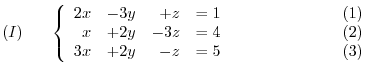
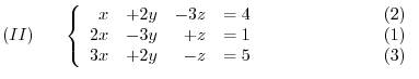
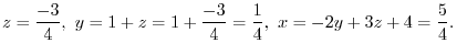
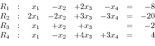
Give a system of the linear equations.
 and
and  . Then we have
Next we multiply the equation by  and add it to . Also multiply the equation by
  and add to
  . Then we have
 by
by
 to make the leading element 1.
 by
by  and add it to the equation
 . Then we have
 thequation and
  th equation:
th equation by a nonzero scalar
th equation:
th equation by a nonzero scalar  th equation by times the th equation plus the th equation.
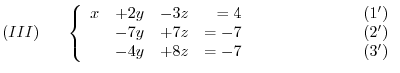
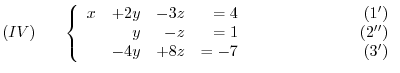
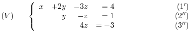
Now we apply elementary operations to the system of linear equations.
First of all,
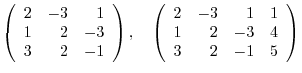
The matrix composed of coefficients of the system of linear equations  is called a coefficient matrix. The matrix composed of coefficient matrix and constant terms is called an augmented matrix and denoted by
 |
|||
 |
 |
||
 |
 |
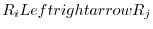
 : Interchange the th row and th row:
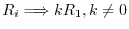
 : Multiply the th row by a nonzero scalar :
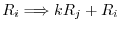
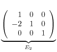
 : Replace the th row by times the th row plus the th row:
Generally, those 3 operations on a metrix  is called fundamental row operation.
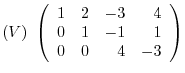
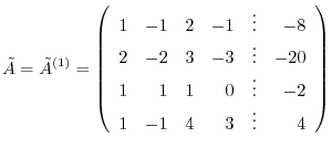
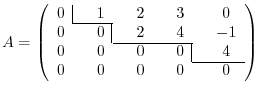
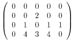
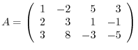
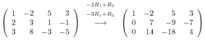
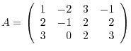
Answer The augmented matrix is given by
 . Then we have
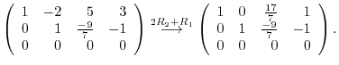
Now the Pivot element
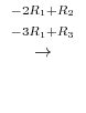
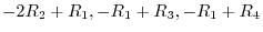
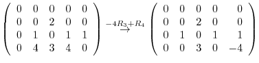
 . So, use the elementary operation
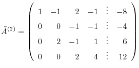
 . Then
 is already eliminated from
  . Thus,
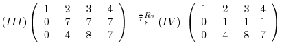
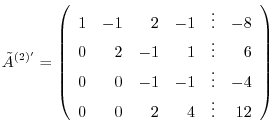
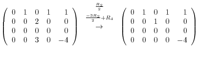
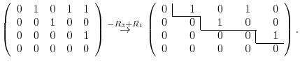
 . Continue elementary operation such as
 . Then
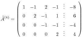
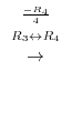
Thus, we have
 |
 |
 |
|
 |
|
 |
|
 |
|
 |
|
 |
|
 |
If a matrix  is created by appling finitely many elementary operation on , a matrix is said to be row equivalent and denoted by
  . If elmentary operation
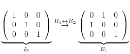
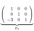
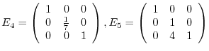
 or is applied once to the identity matrix of the order
  , then the matrix obtained is called a fundamental matrix. You might already have noticed that an elementary operation can be written using an elementary matrix. For example, the elementary operation from to
  is
is
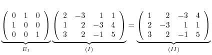
 and the corresponding elementary matrix can be obtained by applying the elementary operation
on
and the corresponding elementary matrix can be obtained by applying the elementary operation
on  .
.
 to from the left. Then we have
 is given by the following:
 is given by the following:
 . Thus,
 's to the matrix from the left. Then
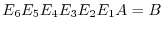 and are row equivalent..
When you apply elementary operations on a matrix . we are able to obatin a matrix so that all entries below the diagonal are zero. We say this matrix as upper triangular matrix.
 , it is called arow reduced echelon matrix and denoted by
  . We show next that every matrix is row equivalent to a row reduced echlon matrix.
Proof It is up to you..
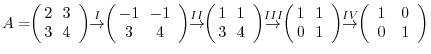
Answer
 |
|||
 |
 |
||
 |
 |

In this example, the order of the row operation is not important.
and  are row reduced echlon matrix and row equivalent to , then
  .
.
Proof It is up to you.
It is important to know that the matrix row equivalent to is unique.
 Rank of matrix
The number of steps of the row reduced echlon form is important for application. This number is called the rank of a matrix and denoted by
 . For example, the rank of 2.2 is
  .
.
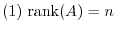
be a square matrix of the order . Then the followings are equivalent.

Proof
If
 , then the rank of is . Thus,
 .
.
Conversely, if
, then the number of steps of the row reduced matrix of is . By the definition of the row reduced echlon matrix, the first nonzero entry is . Then every diagonal element is . Thus,
.
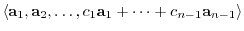
The rank of a matrix can be defined by the concept of a vector space.
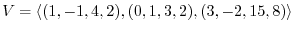
 are elements of
 . Then a linear combination of these vectors is defined as follows:
 is then a subspace of
(Example1.4). This vector space is called a row space or row spanned subspace of . Now let
is then a subspace of
(Example1.4). This vector space is called a row space or row spanned subspace of . Now let
 . Then
 |
|
 |
|
|
 |
||
|
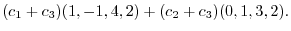 |
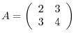
 . Furthermore,
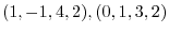
 and
and  are linearly independent. Thus, these two vectors a basis of this row space. This shows that the dimension of the row space of is
  . We now find the row reduced echlon matrix of . Then
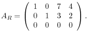
 . Thus in this example,
Proof
Let be a matrix of
 . Let the row vectors of
 be
be
 . A row space is alinear combination of

 has no effect on the linear combination. Thus, it will not have any effect on the dimension of the row space.
Next, we use to find the row reduced echlon matrix. Suppose that
 is a linear combination of
 , then
 and
and
 are the same. This corresponds to zeor row vector in the row echlon matrix and removing the row vector
. Repeating this process, we can find the row vector
are the same. This corresponds to zeor row vector in the row echlon matrix and removing the row vector
. Repeating this process, we can find the row vector
 corresponding to the row reducing. The row vectors are linealy independent. Thus the dimension of the row vectors is the same as the rank of row reduced matrix.
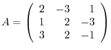
The rank of a matrix plays an important role on solving the system of linear equations. Befor moving to the next section, try to solve the system of linear equations.
.
Answer
 |
|
 |
|
 |
 |
is . Thus
.
We note that the row vectors
 and
and
 of the matrix forms a basis of the row space of . Thus the dimension of the row space is ..
1. Find the row reduced matrix which is row equivalent to
 .
.
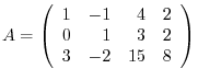
2. Find the rank of the following matrices.
3. Given
 . Apply elmentary operations
 .
.
 . Show the matrix
  as a product of the matrix and elementary matrices.
4.
 can be reduced to the identiry matrix by using the elementary row operation. Find the product of matrices
  so that
  .
.
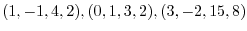
5. Find the dimension of the subspace spanned by the following vectors.