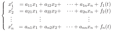
Next: Exercise Up: Systems of differential equations Previous: Systems of differential equations Contents Index
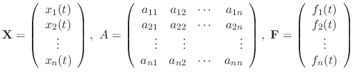
 and the column vector
  anf
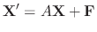
anf  , we can express
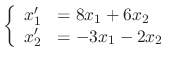
The differentiable functions
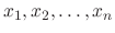 satisfying the above equation is called the solution. When
 , we say that the differential equation is homogeneous equation.
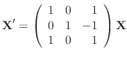
We will explain how to solve
 .
Let
.
Let
 . Then
 , we have

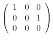
 denotes the unit matrix of the degree
  .
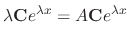
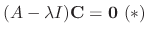
Now if
.
Now if
 , then the equation is obviously satisfied. So, we need to find the
 satisfying the above equation.
Note that if
satisfying the above equation.
Note that if
 , then
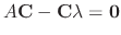
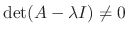
 . Thus to find the
, we have to solve
. Thus to find the
, we have to solve
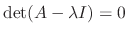 .
The
.
The  is called the eigenvalue of the matrix and the nonzero C satisfying
 is called the eigenvector for .
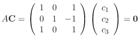
SOLUTION
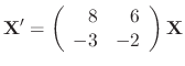
Let
 . Then we have
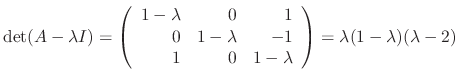
 .
Now we find the eigenvector for
.
Now we find the eigenvector for
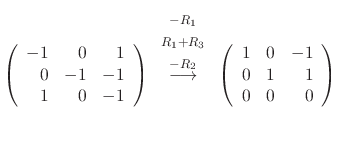
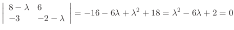
 . Substitute
into the equation (*). Then
. Substitute
into the equation (*). Then
 |
 |
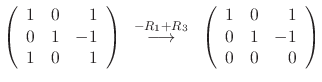 |
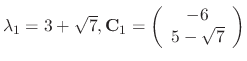
 . Then
 ,
,  Thus, the eigenvector C is
 and
and
 is a solution.
 .
.
 |
|
 |
|
 |
 |
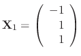
 . Then
  ,
,  and the eigenvector is
 .
.
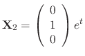 is a solution. Similarly, we find the eigenvector corresponds to

 |
|
 |
 and
and
 . Thus the eigenvector is
 .
.
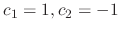
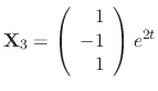 is a solution. Since
 are linearly independent, we have
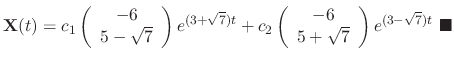
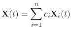
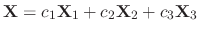 and the general solution is
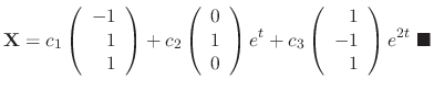
has the different eigenvalues
 and corresponding eigenvectors
 . Then the general solution is given by
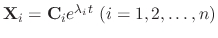 are the solutions of
and linearly independent.
are the solutions of
and linearly independent.
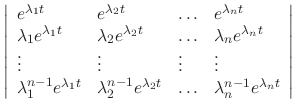
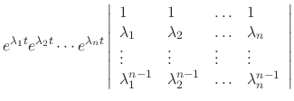
Proof
 |
|
 |
|
|
 |
||
|
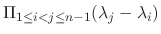 |
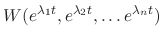
 are different,
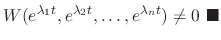
The linearly independent solutions of
is called the fundamental solution.
 .
.
SOLUTION
 |
|
 |
|
 |
|
 |
 .
For
.
For
 .
For
.
For
 . Thus the general solution is